Random Forests and Gradient Boosted Trees in TensorFlow
Contents
Random Forests and Gradient Boosted Trees in TensorFlow#
In this project/tutorial, we will
Visualise the Stroke Prediction Dataset with a parallel coordinate plot
Use TensorFlow Decision Forests (TF-DF) to train a random forest and a gradient boosted trees model to do binary classification
Compare the performance of the tree models against the neural network trained in the previous tutorial Binary Classification with the Stroke Prediction Dataset
In TensorFlow version 2.5.0, support for decision trees and forests was added and announced during Google I/O 2021. The documentation, including guides, tutorials and the API reference can be found here. TensorFlow Decision Forests (TF-DF) includes the models
which we are going to explore in this tutorial.
Installation#
As of now, TensorFlow Decision Forests is not yet available on Anaconda
and instead has to be installed from the Python Package Index via pip.
Combining package installations via conda and pip should be done with a
certain level of care. Following spellbook’s typical setup specified in
spellbook.yml and combining the normal conda-based TensorFlow
installation with TF-DF installed via pip will most probably not work.
Instead, we are going to create a separate conda environment
spellbook-no-tensorflow just for this tutorial and install both
TensorFlow and TF-DF via pip using the provided requirements.txt.
So let’s roll:
$ cd examples/2-tensorflow-decision-forests
If the default spellbook conda environment is currently active,
deactivate it
$ conda deactivate
and create the dedicated environment excluding TensorFlow
$ conda env create --file spellbook-no-tensorflow.yml
Once this is done, activate it and use pip to install both TensorFlow
and TensorFlow Decision Forests into the new conda environment
spellbook-no-tensorflow
$ conda activate spellbook-no-tensorflow
$ pip install -r requirements.txt
Parallel Coordinate Plots#
This tutorial uses Kaggle’s Stroke Prediction Dataset,
just like the Binary Classification with the Stroke Prediction Dataset project before.
So therefore, before we try out the decision trees in TF-DF, let’s have
a look at another possibility of visualising entire datasets in a rather
compact way - parallel coordinate plots. In spellbook, they are
implemented in spellbook.plot.parallel_coordinates() and can be used
like this:
fig = sb.plot.parallel_coordinates(data.sample(frac=1.0).iloc[:500],
   features, target, categories)
sb.plot.save(fig, 'parallel-coordinates.png')
We first shuffle the datapoints using pandas.DataFrame.sample() and
then take the first 500 of them in order to get a
representative subset of all patients. The resulting plot is shown in
Figure 1.
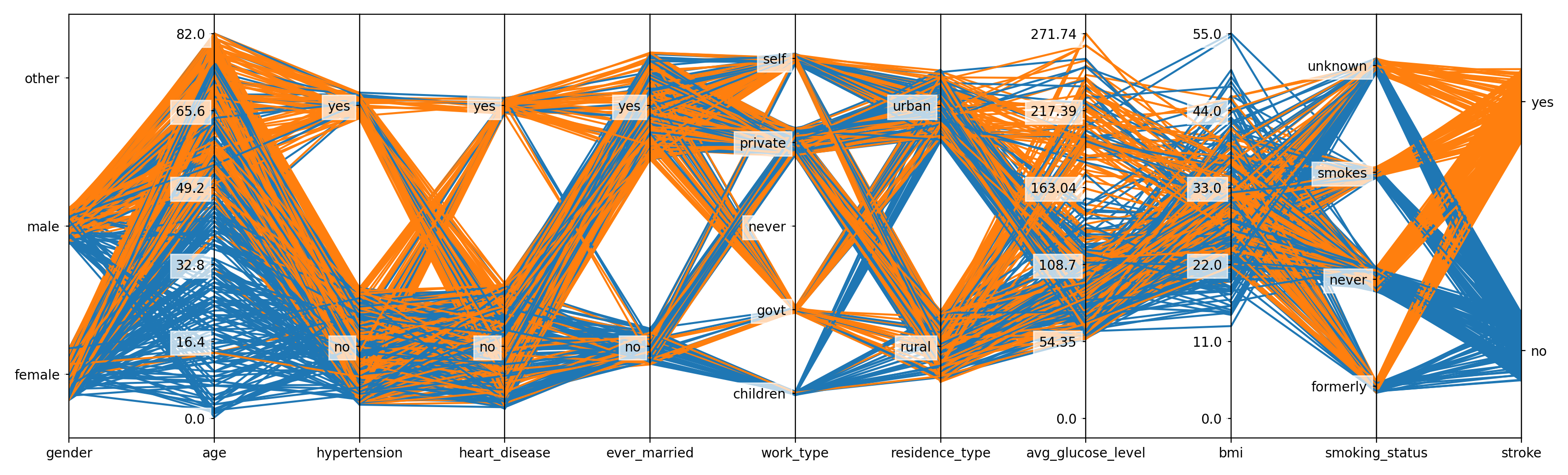
Figure 1: Parallel coordinates plot showing a subset of Kaggle’s Stroke Prediction Dataset# |
We can see the binary categorical target variable stroke on the far
right-hand side of the plot. Patients with a stroke are shown with orange
lines and patients without a stroke with blue lines. The features are shown
in individual coordinate axes left of the target. There are both continuous
variables, such as age or bmi, and categorical variables, such as
gender or heart_disease and the density of the lines indicates the
prevalence of the target labels. Looking at the age of the patients, we can
see that strokes are more present at higher ages.
For categorical variables, the datapoints are randomly
smeared or shifted around the respective categories or classes. Therefore,
the lines are not all drawn exactly on top of each other and it is possible
to get an impression of the composition of the datapoints in a certain category
in terms of the target labels. For instance, we can see that the no
classes of the variables hypertension and heart_disease contain
significant fractions of patients both with and without strokes, while the
yes categories seem to be enriched in stroke patients. This seems
plausible as it indicates positive correlations between these conditions
and the presence of strokes. Additionally, the size of the smearing or
shifting interval is chosen in proportion to the number of datapoints in
the respective categories. Therefore, it is possible to get a feeling for
how many patients fall into which class for each feature. For example, we
can see that more patients work in the private sector that for the
government.
Random Forest#
Just like regular TensorFlow, TF-DF implements the Keras API and therefore, we can follow very closely what we did in Binary Classification with the Stroke Prediction Dataset. So now let’s start using TF-DF and begin with the random forest model:
# data loading and cleaning
data, vars, target, features = helpers.load_data()

# inplace convert string category labels to numerical indices
categories = sb.input.encode_categories(data)

# oversampling (including shuffling of the data)
data = sb.input.oversample(data, target)

# split into training and validation data
n_split = 7000
train = tfdf.keras.pd_dataframe_to_tf_dataset(
    data[features+[target]].iloc[:n_split], label=target)
val = tfdf.keras.pd_dataframe_to_tf_dataset(
    data[features+[target]].iloc[n_split:], label=target)
After loading the Stroke Prediction Dataset with the helper function, we apply oversampling to counteract the imbalance in the target classes between the 4.3% of the patients with a stroke and the overwhelming majority of 95.7% without a stroke. The dataset and the method of oversampling are described in detail in Binary Classification with the Stroke Prediction Dataset. Finally, we split the dataset into a training and a validation set using TF-DF’s tfdf.keras.pd_dataframe_to_tf_dataset.
Note that we hardly did any preprocessing - in particular, decision trees do
not need normalised data. Likewise, it is not necessary to turn categorical
variables expressed by strings or integers into properly indexed
pandas.Categoricals. This is only needed here for the oversampling
to work - but not for the decision trees.
Next, we prepare a range of metrics useful for binary classification - the same
ones that are also used and described in
Model Training and Validation.
Afterwards, we instantiate a tfdf.keras.RandomForestModel,
sticking to the default values. We add the metrics using the compile method
and train the model with model.fit on the training dataset train.
Finally, we save the model so that it can be reloaded and used again later:
# define binary metrics
metrics = [
    tf.keras.metrics.BinaryCrossentropy(name='binary_crossentropy'),
    tf.keras.metrics.BinaryAccuracy(name='accuracy'),
    tf.keras.metrics.TruePositives(name='tp'),
    tf.keras.metrics.TrueNegatives(name='tn'),
    tf.keras.metrics.FalsePositives(name='fp'),
    tf.keras.metrics.FalseNegatives(name='fn'),
    tf.keras.metrics.Recall(name='recall'),
    tf.keras.metrics.Precision(name='precision')
]

# prepare and train the model
model = tfdf.keras.RandomForestModel()
model.compile(metrics=metrics)
model.fit(train)
# model.summary()
model.save('model-{}'.format(prefix))
By default, tfdf.keras.RandomForestModel uses 300 trees with a depth of
up to 16 and fitting our training dataset only takes a few seconds. The
rapid way of evaluating the model performance goes somewhat like this:
eval = model.evaluate(val, return_dict=True)
print('eval:', eval)
eval is a dict containing the values of the metrics calculated
from the validation dataset.
But let’s go on and calculate the confusion matrix:
# separate the datasets into features and labels
train_features, train_labels = zip(*train.unbatch())
val_features, val_labels = zip(*val.unbatch())

# obtain the predictions of the model
train_predictions = model.predict(train)
val_predictions = model.predict(val)

# not strictly necessary: remove the superfluous inner nesting
train_predictions = tf.reshape(train_predictions, train_predictions.shape[0])
val_predictions = tf.reshape(val_predictions, val_predictions.shape[0])

# until now the predictions are still continuous in [0, 1] and this breaks the
# calculation of the confusion matrix, so we need to set them to either 0 or 1
# according to an intermediate threshold of 0.5
train_predicted_labels = sb.train.get_binary_labels(
    train_predictions, threshold=0.5)
val_predicted_labels = sb.train.get_binary_labels(
    val_predictions, threshold=0.5)

# calculate and plot the confusion matrix
class_names = list(categories['stroke'].values())
class_ids = list(categories['stroke'].keys())
val_confusion_matrix = tf.math.confusion_matrix(
    val_labels, val_predicted_labels, num_classes=len(class_names))
sb.plot.save(
    sb.plot.plot_confusion_matrix(
        confusion_matrix = val_confusion_matrix,
        class_names = class_names,
        class_ids = class_ids),
    filename = '{}-confusion.png'.format(prefix))
Just like in Model Training and Validation, we can also plot normalised versions of the confusion matrix. The confusion matrix with the absolute datapoint numbers is given in Figure 2 and a version where each true label/class is normalised in Figure 3:
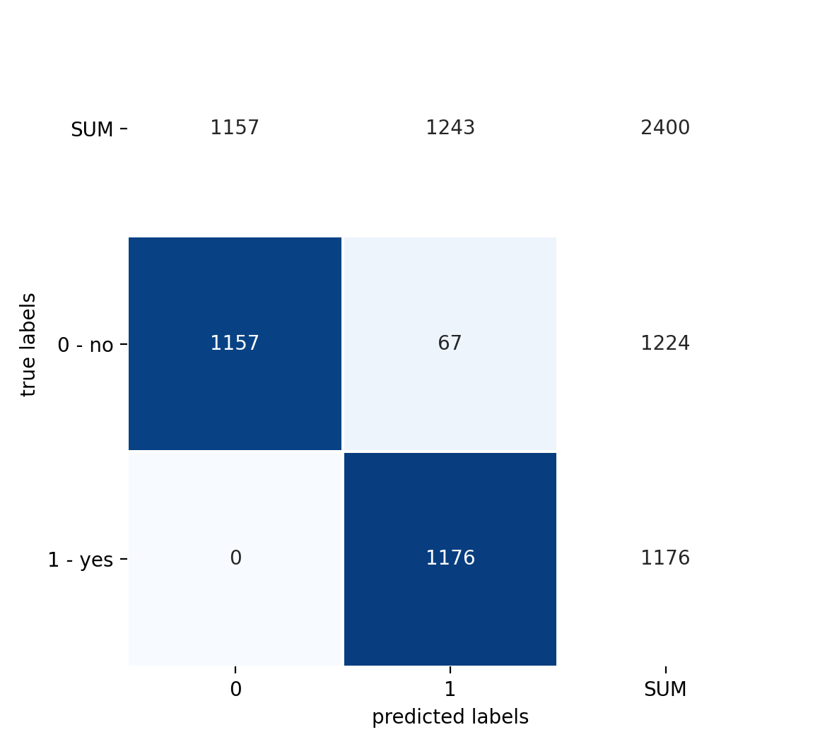
Figure 2: Confusion matrix with absolute datapoint numbers# |
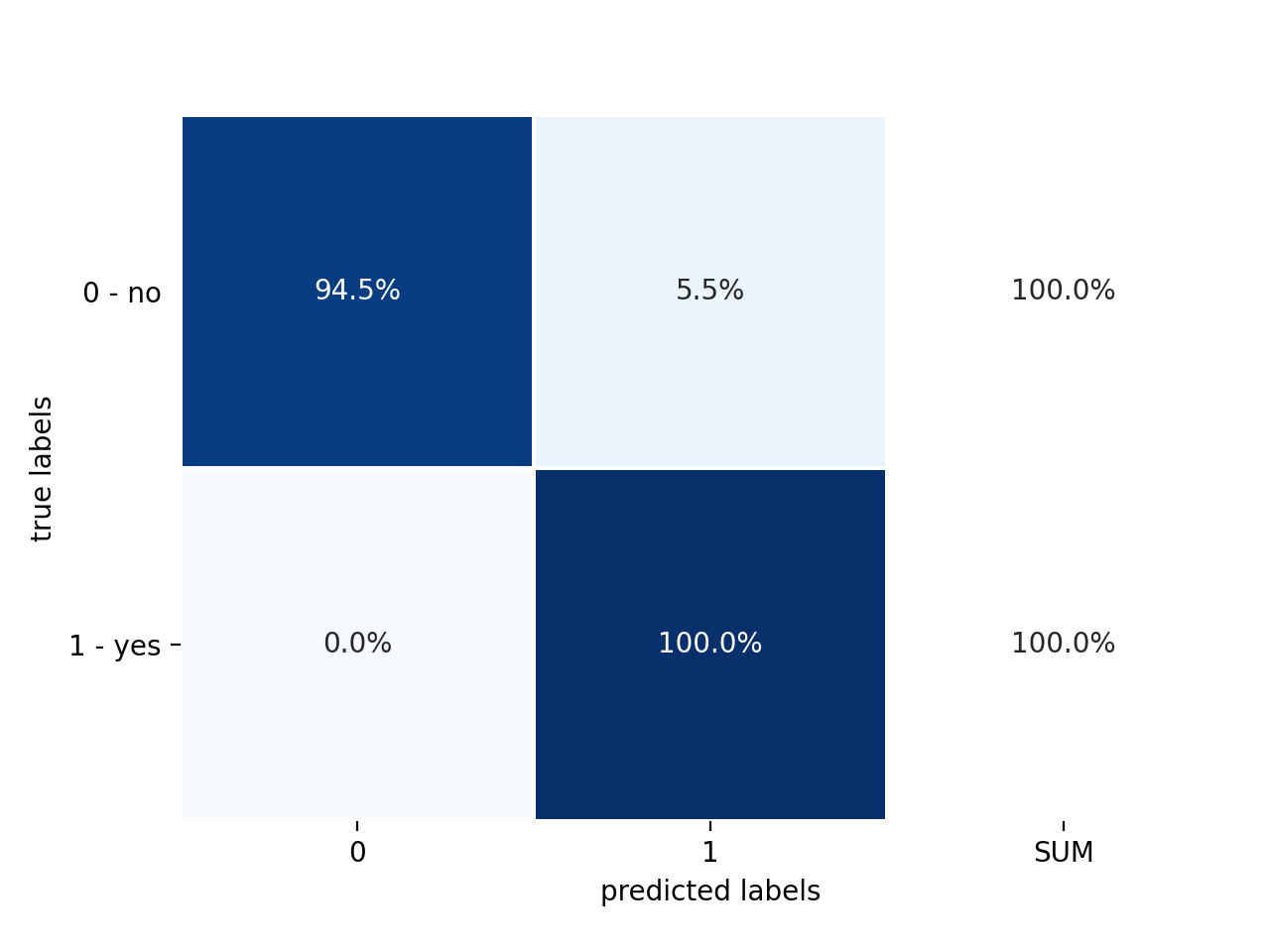
Figure 3: Confusion matrix normalised along each true label/class# |
We can see that already with the default forest configuration, the model’s performance is good enough to not produce any false negatives. As for the false positives, only 5.5% of the truly negative datapoints are wrongly classified as positive.
Gradient Boosted Trees#
Random forests consist of many trees, each trained on a randomly drawn subset of the full training dataset. In contrast, a boosted decision trees model consists of many trees, where after training one tree, the weights of the wrongly classified datapoints are increased before training the next tree. This way, increasingly more importance is puts on datapoints that are hard to classify.
The only real change we have to make to use a gradient boosted trees model is in the instantiation:
model = tfdf.keras.GradientBoostedTreesModel()
By default, TF-DF trains up to 300 trees with a depth of up to 6.
The resulting confusion matrices are shown in Figure 4 and 5:

Figure 4: Confusion matrix with absolute datapoint numbers# |

Figure 5: Confusion matrix normalised along each true label/class# |
We can see that the performance is very similar to the random forest, with a false positive rate (FPR) of 5.8%.
Before we go on to compare the different tree models and the final neural
network classifier trained in
Binary Classification with the Stroke Prediction Dataset,
let’s have a look at a model-agnostic way of determining the importance
that each feature plays in the performance of the classifier: the
permutation importance. While one or more input features cannot simply
be removed, the idea behind permutation importance is to break the
correlation of a feature with the target by randomly permuting the values
of just that particular feature - hence the name. This way, the classifier
is no longer able to use that feature when deriving the prediction.
Permutation importance is implemented in spellbook in
spellbook.inspect.PermutationImportance, based on
sklearn.inspection.permutation_importance(), and can be calculated
and plotted as follows for any of the metrics previously defined and passed
to the model in the compile step:
importance = sb.inspect.PermutationImportance(
   data, features, target, model, metrics, n_repeats=10, tfdf=True)
sb.plot.save(
   importance.plot(
      metric_name='accuracy',
      annotations_alignment = 'left',
      xmin = 0.62),
   filename='{}-permutation-importance-accuracy.png'.format(prefix))
resulting in the plot shown in Figure 6:
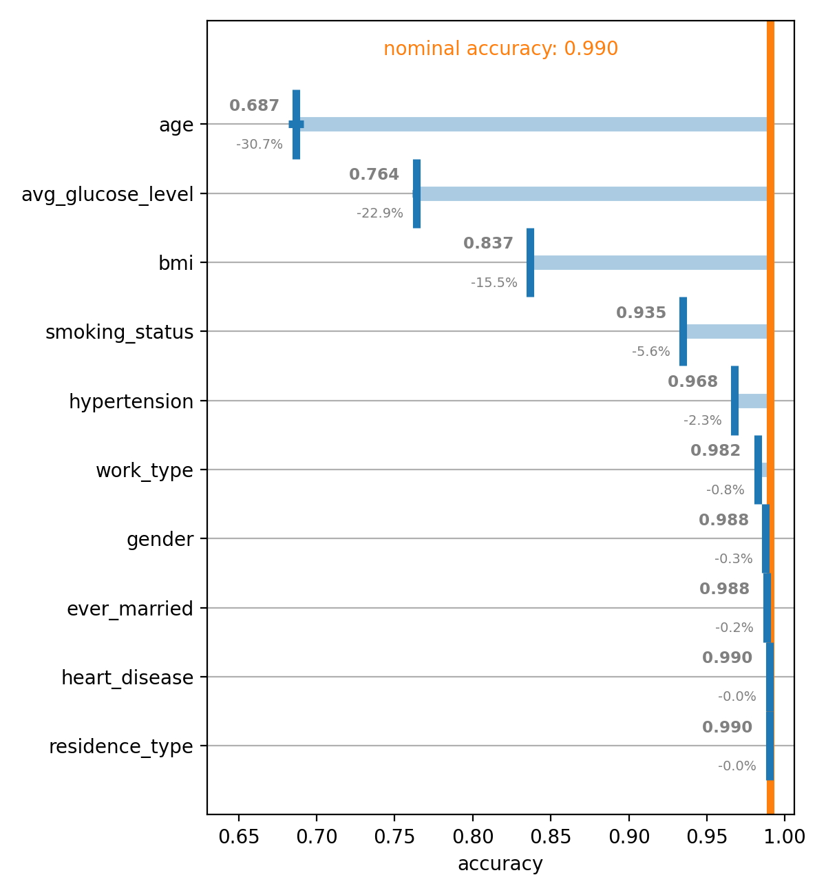
Figure 6: Permutation importance# |
We can see to what values the metric, in this case the classification accuracy,
decreases when each one of the feature variables is randomly permuted. Each
feature is permuted n_repeats times and the average and standard
deviation of the resulting metrics are calculated. The standard deviations
are used to draw horizontal error bars on the average deteriorated metrics,
but can also be printed into the plot.
We can see that the gradient boosted trees classifier relies most heavily on age, the average glucose level and the BMI, with the accuracy dropping by about 31%, 23% and 16%, respectively, when the corresponding values are scrambled.
While the approach behind permutation importance is model-agnostic, care
has to be taken in interpreting the results when some of the features are
correlated. In this case, information from the missing permuted feature
can at least partly be recovered by the classifier from the remaining
correlated variable(s), leading to a less-than-expected deterioration
of the studied metric. To overcome this limitation,
spellbook.inspect.PermutationImportance provides a mechanism for
grouping multiple features into clusters and permuting them simultaneously.
Further info:
Comparison Against Neural Networks#
Finally, let’s compare our tree classifiers against the final neural network classifier trained at the end of Binary Classification with the Stroke Prediction Dataset using both oversampling and input normalisation and have a look at the different Receiver Operator Characteristic (ROC) curves:
import spellbook as sb

# load the pickled ROC curves of the different models
roc_network = sb.train.ROCPlot.pickle_load(
    '../1-binary-stroke-prediction/oversampling-normalised-e2000-roc.pickle')
roc_forest = sb.train.ROCPlot.pickle_load('random-forest-roc.pickle')
roc_trees = sb.train.ROCPlot.pickle_load('gradient-trees-roc.pickle')

# add and style the ROC curves
roc = sb.train.ROCPlot()
roc += roc_network
roc.curves['oversampling normalised / 2000 epochs (validation)']['line'].set_color('black')
roc.curves['oversampling normalised / 2000 epochs (training)']['line'].set_color('black')
roc += roc_trees
roc.curves['gradient trees (validation)']['line'].set_color('C1')
roc.curves['gradient trees (training)']['line'].set_color('C1')
roc += roc_forest

# calculate and draw the working points with 100% true positive rate
WPs = []
WPs.append(roc.get_WP(
    'oversampling normalised / 2000 epochs (validation)', TPR=1.0))
WPs.append(roc.get_WP(
    'gradient trees (validation)', TPR=1.0))
WPs.append(roc.get_WP(
    'random forest (validation)', TPR=1.0))
roc.draw_WP(WPs, linecolor=['black', 'C1', 'C0'])

# save the plot
sb.plot.save(roc.plot(xmin=-0.2, xmax=11.0, ymin=50.0), 'roc.png')
The resulting ROC curves with the working points at 100% true positive rate (TPR) indicated are shown in Figure 7.
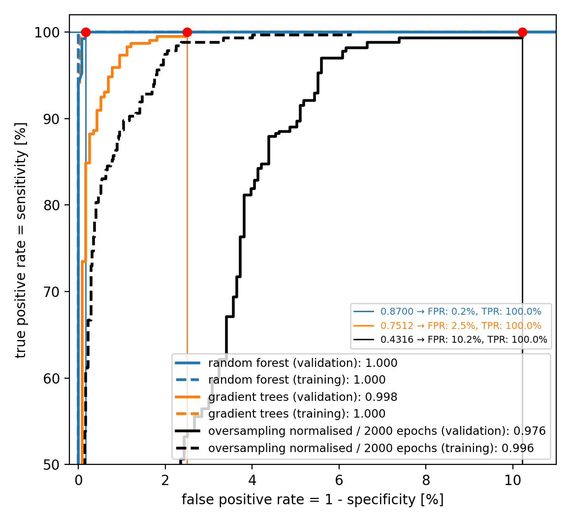
|
There, we can see that both the decision forest and the gradient boosted trees outperform the neural network model, reaching lower false positive rates (FPR) of 0.2% and 2.5%, respectively, while maintaining 100% TPR. Let’s also keep in mind that this is not only without any hyperparameter tuning but even just using the defaults. Furthermore, while it took about an hour to train the neural network classifier on a fairly standard laptop, fitting the decision tree models was a matter of a few seconds.
This illustrates that decision trees tend to prefer structured data, i.e. data showing its characteristic patterns when represented in a table with the features in the columns and each datapoint in a row. While images, being a typical example of unstructured data, can also be represented in such a tabular manner, with each pixel in its own column, this is not a representation geared towards showing the characteristic patterns - which can e.g. move across the image and therefore from some columns to others. Neural networks are better at identifying and learning the relevant patterns in such unstructured datasets.