spellbook.train#

Functions for model training and validation

Classes:

`BinaryCalibrationPlot`(labels, predictions[, ...])	Plot showing calibration/reliability curve(s) in binary classification
`ModelSavingCallback`([foldername, step])	Callback that intermittently saves the full model during training
`ROCPlot`()	Plot containing Receiver Operator Characteristic (ROC) curves and working points (WP)

Functions:

`get_binary_labels`(predictions[, threshold])	Apply threshold to calculate the labels from the predictions
`plot_history`(history[, nrows, ncols, ...])	Plot the timeline of training metrics
`plot_history_binary`(history[, name_prefix])	Convenience function for plotting binary classification metrics

Classes#

BinaryCalibrationPlot#

class spellbook.train.BinaryCalibrationPlot(labels, predictions, names=None, bins=10, plot_args={}, predictions_hist_args={}, predictions_ymin=None, predictions_ymax=None, predictions_yscale=None)[source]#

Plot showing calibration/reliability curve(s) in binary classification

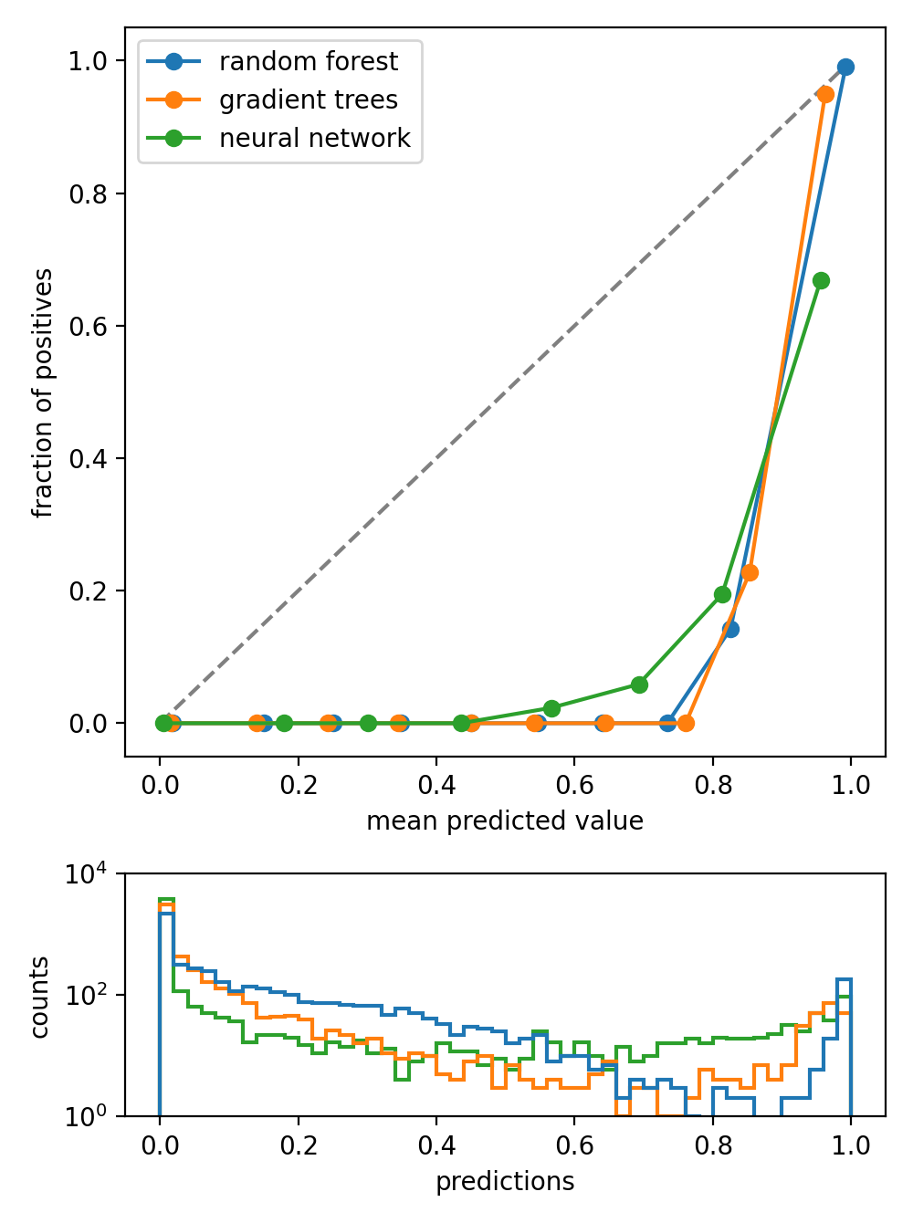
For each classifier, whose calibration curve is to be plotted, a set of true labels and predictions/scores has to be given. The calibration curves are calculated with sklearn.calibration.calibration_curve(): The range of the predictions/scores is divided into bins bins. In each bin, the average of the predictions in that bin is calculated (mean predicted value) as well as the which fraction of the datapoints in that bin is actually positive (fraction of positives). For a perfectly calibrated classifier, the predictions/scores actually give the probabilities for a particular datapoint to belong to the positive class and therefore, the mean predicted values and the fraction of positives are close to each other, resulting in a straight diagonal calibration curve.

Below the calibration curves, histograms of the predictions are shown. It is possible to use a logarithmic y-axis, which can be handy to visualise predictions that are very non-uniformly distributed.

Parameters

labels (array-like or list of array-like) –
The true target labels/classes. The type can be
- numpy.ndarray or tf.Tensor: when plotting a single calibration curve
- list[numpy.ndarray] or list[tf.Tensor]: when plotting one or more calibration curves
predictions (array-like or list of array-like) –
The predicted labels/classes. The type can be
- numpy.ndarray or tf.Tensor: when plotting a single calibration curve
- list[numpy.ndarray] or list[tf.Tensor]: when plotting one or more calibration curves
names (str or list[str]) –
The names of the legend entries for each calibration curve. The type can be
- str: when plotting a single calibration curve
- list[str]: when plotting one or more calibration curves
bins (int or list[int]) –
The number of bins in which to evaluate the calibration, i.e. the fractions of positives vs. the mean predicted values. The type can be
- int: when plotting a single calibration curve
- list[int]: when plotting one or more calibration curves
predictions_hist_args (dict) – Arguments passed on to matplotlib.axes.Axes.hist() when plotting the histograms of the predictions
predictions_ymin (typing.Optional[float]) – The lower end of the y-axis of predictions histogram
predictions_ymax (typing.Optional[float]) – The upper end of the y-axis of predictions histogram
predictions_yscale (typing.Optional[str]) – The scaling behaviour of the y-axis of predictions histogram as described in matplotlib.axes.Axes.set_yscale(). Meaningful values for histograms are 'linear' and 'log'.

fig#: The matplotlib.figure.Figure object holding the plot

grid#: The matplotlib.gridspec.GridSpec object

ax_calibrations#: The matplotlib.axes.Axes object holding the calibration curves

ax_predictions#: The matplotlib.axes.Axes object holding the histograms of the predictions

ModelSavingCallback#

class spellbook.train.ModelSavingCallback(foldername='model', step=10)[source]#

Callback that intermittently saves the full model during training

The model is saved as a folder intermittently in configurable steps during training as well as at the end of the training. The foldername is kept unchanged as training goes on, thus always replacing the last/old model with the current/new state.

Methods:

`__init__`([foldername, step])	Callback that intermittently saves the full model during training
`on_epoch_end`(epoch, logs)	Called at the end of every epoch: Save the model every self.step epochs
`on_train_end`(logs)	Called at the end of the training: Save the model

__init__(foldername='model', step=10)[source]#

Callback that intermittently saves the full model during training

Parameters

foldername (str) – The model is saved as a folder with this name
step (int) – The model is saved every step number of epochs

Returns

An instance of the callback, which is then to be added to the callbacks parameter of tensorflow.keras.Model.fit()

on_epoch_end(epoch, logs)[source]#

Called at the end of every epoch: Save the model every self.step epochs

Parameters

epoch (int) – Index of the epoch
logs (dict) – Metrics for this training epoch as well as the validation epoch if validation is performed. Validation result keys are prefixed with 'val_'.

Return type

None

on_train_end(logs)[source]#

Called at the end of the training: Save the model

Parameters: logs (dict) – Currently the output of the last call to on_epoch_end() is passed to this argument for this method but that may change in the future.
Return type: None

used in#

Serving TensorFlow Models in Docker

Serving *TensorFlow* Models in *Docker*

ROCPlot#

class spellbook.train.ROCPlot[source]#

Plot containing Receiver Operator Characteristic (ROC) curves and working points (WP)

Methods:

`__iadd__`(other)	The `+=` operator
`__init__`()
`add_curve`(name, labels, predictions[, plot_args])	Add a ROC curve
`draw_WP`(WP[, line, linestyle, linecolor, ...])	Draw one or more working points and indicate their classifier thresholds as well as true positive and false positive rates
`get_WP`(curve_name[, threshold, FPR, TPR, method])	Find working point(s) at specified classifier threshold(s), TPR(s) or FPR(s)
`get_legend_labels`()	Get the labels / texts for the ROC curves to be shown in the legend
`get_legend_lines`()	Get the lines representing the ROC curves to be shown in the legend
`pickle_load`([filename])	Unpickle and load an instance/object from a file
`pickle_save`([filename])	Pickle this instance/object and save it to a file
`plot`([xmin, xmax, ymin, ymax])	Plot one or more ROC curves and working points to a figure object
`remove_curve`(name)	Remove a ROC curve
`rename_curve`(old_name, new_name)	Change the name of a ROC curve

__iadd__(other)[source]#

The += operator

Return type: spellbook.train.ROCPlot

__init__()[source]#

add_curve(name, labels, predictions, plot_args={})[source]#

Add a ROC curve

Internally it uses sklearn.metrics.roc_auc_score() to calculate the ROC curve from the true labels and the predictions / classifier outputs.

Parameters

name (str) – The name of the ROC curve
labels ([float] / numpy.ndarray(ndim=1)) – The target labels for the datapoints
predictions ([float] / numpy.ndarray(ndim=1)) – The sigmoid- activated predictions for the datapoints. Note that not the predicted labels but rather the sigmoid-activated predictions should be used so that by scanning different thresholds the different true positive / false positive rates can be determined.
plot_args (dict) – Arguments to be passed to matplotlib.axes.Axes.plot()

Return type

None

draw_WP(WP, line=True, linestyle='-', linecolor='C0', info=None, highlight=None)[source]#

Draw one or more working points and indicate their classifier thresholds as well as true positive and false positive rates

Parameters

WP (dict / [dict]) – One or more working points as returned by get_WP()
linestyle (str / [str], optional) – Linestyle(s) for drawing the horizontal and vertical lines designating the working point(s)
info (bool / [int], optional) – Whether or not the parameters of the WP(s) should be shown on the graph. If None or True, then all WPs are included. If False or [], none are given. If a list of integers is given, then the WPs with the corresponding indices are shown.
highlight (bool / int, optional) – Whether or not and which WP and its parameters should be highlighted. If a single WP is given, then highlight should be a bool. If multiple WPs are given, it should be an integer specifying the index of the WP to highlight.

Some examples of how to calculate and draw working points are given here in get_WP().

Return type: None

get_WP(curve_name, threshold=None, FPR=None, TPR=None, method='interpolate')[source]#

Find working point(s) at specified classifier threshold(s), TPR(s) or FPR(s)

Either the classifier threshold, the TPR or the FPR parameter can be specified to determine one or more matching working points (WP), but not more than one of the three at the same time.

Parameters

curve_name (str) – Name of the curve from which to determine the WP(s)
threshold (float / [float]) – Threshold/cut value on the classifier’s sigmoid-activated output to separate the two classes
FPR (float / [float]) – Target FPR(s) to match
TPR (float / [float]) – Target TPR(s) to match
method (interpolate / nearest) –
Method for determining the working point(s)
- interpolate: find the two points that enclose the target value and interpolate linearly between them
- nearest: find the point that is nearest to the target value

Returns

If threshold/FPR/TPR is a scalar, then a dict containing the matching WP with its threshold, FPR and TPR is returned. If threshold/FPR/TPR is a list, then a list of dicts is returned, with each entry in the list corresponding to one WP.

Return type

dict / [dict]

Example

Get a single working point by specifying a classifier threshold and draw it

roc = sb.train.ROCPlot()
roc.add_curve('1000 epochs (testing)',
              test_labels, test_predictions.numpy(),
              plot_args = dict(color='C0', linestyle='-'))
WP = roc.get_WP('1000 epochs (testing)', threshold=0.5)
roc.draw_WP(WP, linecolor='C0')
fig = roc.plot()
sb.plot.save(fig, 'roc.png')

Get multiple working points by specifying FPRs and TPRs and draw them

roc = sb.train.ROCPlot()
roc.add_curve('1000 epochs (testing)',
              test_labels, test_predictions.numpy(),
              plot_args = dict(color='C0', linestyle='-'))
WPs1 = roc.get_WP('1000 epochs (testing)', FPR=[0.1, 0.2])
WPs2 = roc.get_WP('1000 epochs (testing)', TPR=[0.8, 0.9])
roc.draw_WP(WPs1+WPs2, linecolor=['C0', 'C1', 'C2', 'black'])
sb.plot.save(roc.plot(), 'roc.png')

get_legend_labels()[source]#

Get the labels / texts for the ROC curves to be shown in the legend

Returns: Labels / texts for the ROC curves to be shown in the legend
Return type: [str]

get_legend_lines()[source]#

Get the lines representing the ROC curves to be shown in the legend

Returns: Lines representing the ROC curves to be shown in the legend
Return type: [matplotlib.lines.Line2D]

classmethod pickle_load(filename='roc.pickle')[source]#

Unpickle and load an instance/object from a file

Based on https://stackoverflow.com/q/35649603 and https://stackoverflow.com/a/35667484

Parameters: filename (str) – The name of the file from which the object should be loaded
Returns: The unpickled instance / object
Return type: ROC

pickle_save(filename='roc.pickle')[source]#

Pickle this instance/object and save it to a file

Based on https://stackoverflow.com/q/35649603 and https://stackoverflow.com/a/35667484

Parameters: filename (str) – The name of the file to which the object should be saved
Return type: None

plot(xmin=0.0, xmax=100.0, ymin=0.0, ymax=102.0)[source]#

Plot one or more ROC curves and working points to a figure object

Parameters

xmin (float) – Lower end of the x-axis
xmax (float) – Upper end of the x-axis
ymin (float) – Lower end of the y-axis
ymax (float) – Upper end of the y-axis

Returns

The figure containing the full plot including one or more curves and working points

Return type

matplotlib.figure.Figure

remove_curve(name)[source]#

Remove a ROC curve

Parameters: name (str) – The name of the curve to be removed
Return type: None

rename_curve(old_name, new_name)[source]#

Change the name of a ROC curve

Parameters

old_name (str) – The old name
new_name (str) – The new name

Return type

None

Functions#

get_binary_labels#

spellbook.train.get_binary_labels(predictions, threshold=0.5)[source]#

Apply threshold to calculate the labels from the predictions

It is necessary to apply the threshold and unequivocally assign each datapoint to a category for the calculation of the confusion matrix to work correctly in TensorFlow. When given the sigmoid-activated classifier output, the confusion matrix calculation will otherwise floor() the predictions to zero and associate all datapoints with the first/negative class.

Parameters

predictions (typing.Union[numpy.ndarray, tensorflow.python.framework.ops.Tensor]) – The sigmoid-activated classifier outputs, one value for each datapoint
threshold (float) – Datapoints whose prediction is below the threshold are associated to the first/negative class, datapoints whose prediction is above the threshold to the second/positive class

Return type

numpy.ndarray

Returns

Array of predicted labels

Examples:

>>> import numpy as np
>>> import spellbook as sb

>>> predictions = np.arange(0.0, 1.0, 0.2)
>>> print(predictions)
[0.  0.2 0.4 0.6 0.8]

>>> # default threshold of 0.5
>>> predicted_labels = sb.train.get_binary_labels(predictions)
>>> print(predicted_labels)
[False False False  True  True]

>>> # custom threshold of 0.7
>>> predicted_labels = sb.train.get_binary_labels(predictions, 0.7)
>>> print(predicted_labels)
[False False False False  True]

>>> # type(predictions)
>>> predicted_labels = sb.train.get_binary_labels((0.1, 0.5, 0.9))
Traceback (most recent call last):
   ...
TypeError: Argument 'predictions' must be of type 'numpy.ndarray' or 'tensorflow.Tensor'

plot_history#

spellbook.train.plot_history(history, nrows=1, ncols=1, metrics=[['loss', 'val_loss']], names=[['training loss', 'validation loss']], axes=[['l', 'l']], colors='C0', zorders=2.0, scaling_factors=[[1.0, 1.0]], formats=[['.3f', '.3f']], units=[['', '']], titles=[None], y1labels=['loss'], y2labels=['accuracy'], legend_positions=['bl'], fontsize=None, figure_args={})[source]#

Plot the timeline of training metrics

Parameters

history (dict, pandas.DataFrame or tf.keras.callbacks.History) – TensorFlow history object returned by the model training or read from a *.csv file produced with the tf.keras.callbacks.CSVLogger callback during training
nrows (int) – Optional. Number of rows of plots arranged in a grid
ncols (int) – Optional. Number of columns of plots arranged in a grid
metrics ([[str]]) – Optional. Names of the metrics in the history object that should be plotted
names ([[str]]) – Optional. How the plotted metrics should be named in the legends
axes ([[str]]) – Optional. l or r to describe on which y-axis a particular variable should be drawn
colors (str / [[str]]) – Optional. The line color(s). Can be either a single color string, in which case all lines will have this same color, or a list of lists of strings specifying the line colors for each metric.
zorders (float / [[float]]) – Optional. The zorder(s). Can be either a single float, in which case all zorders will have this same value, or a list of lists of floats specifying the zorders for each metric.
scaling_factors ([[float]]) – Optional. Scaling factors that multiply each metric
formats ([[str]]) – Optional. Format strings specifying how last value of each metric should be printed in the legends. Metrics are floats.
units ([[str]]) – Optional. Units that should be appended to the legend entry for each metric
titles ([str]) – Optional. List containing one title for each plot in the grid
y1labels ([str]) – Optional. List containing one label for the left axes for each plot in the grid
y2labels ([str]) – Optional. List containing one label for the right axes for each plot in the grid
legend_positions ([str]) – Optional. List containing a two-character string governing the legend position for each plot in the grid. Possible values are tl, tc, tr, cl, cc, cr, bl, bc and br as implemented in spellbook.plotutils.legend_loc() and spellbook.plotutils.legend_bbox_to_anchor().
fontsize (typing.Optional[float]) – Optional, baseline fontsize for all elements. This is probably the fontsize that medium corresponds to?
figure_args (dict) – Optional, arguments for the creation of the matplotlib.figure.Figure with matplotlib.pyplot.figure()

Returns

The figure containing the plot or grid of plots

Return type

matplotlib.figure.Figure

plot_history_binary#

spellbook.train.plot_history_binary(history, name_prefix='history-binary')[source]#

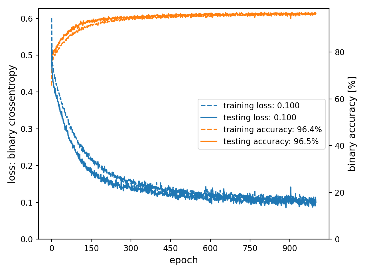
Convenience function for plotting binary classification metrics

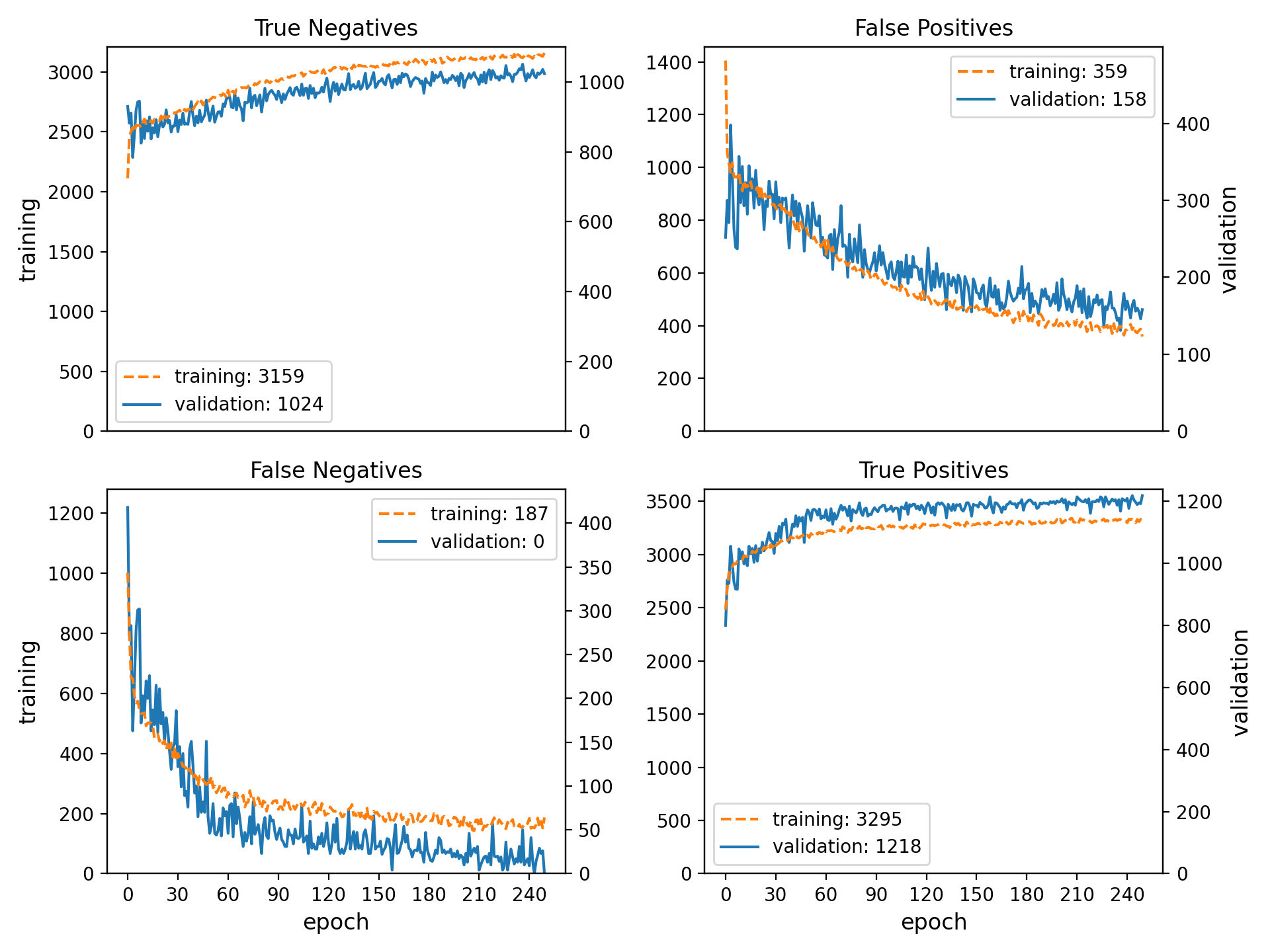
The following plots are generated:

<name_prefix>-loss-acc.png: Loss (binary crossentropy) and accuracy
<name_prefix>-pos-neg.png: Numbers of true/false positives/negatives
<name_prefix>-rec-prec.png Recall/sensitivity and precision

The metrics are defined as:

Recall = Sensitivity = True Positives / (True Positives + False Negatives)
Precision = True Positives / (True Positives + False Positives)

In the plot containing the true/false positives/negatives, the left/primary and right/secondary y-axes are scaled relative to each other according to the ratio of the sizes of the training and validation datasets. Therefore, for a correctly working model and in the absence of significant overtraining, the training and validation curves should lie more or less on top of each other.

Parameters

history (dict, pandas.DataFrame or tf.keras.callbacks.History) – TensorFlow history object returned by the model training or read from a *.csv file produced with the tf.keras.callbacks.CSVLogger callback during training
name_prefix (str) – Prefix to the filenames of the plots

Return type

None

	Contact me on GitHub
	Contact me on LinkedIn

spellbook

spellbook.train

Contents

spellbook.train#

Classes#

BinaryCalibrationPlot#

ModelSavingCallback#

used in#

ROCPlot#

Functions#

get_binary_labels#

plot_history#

plot_history_binary#